Introduction
The position of the detectors with respect to each other and with respect to a radioactive source is very important. To understand the principle of operation of a PET-camera better you will be guided through a simulation program where gamma photons from one or several radioactive sources are absorbed by two detectors. Note that in a real PET-camera tens of thousands of detectors are used. The principle remains the same though.
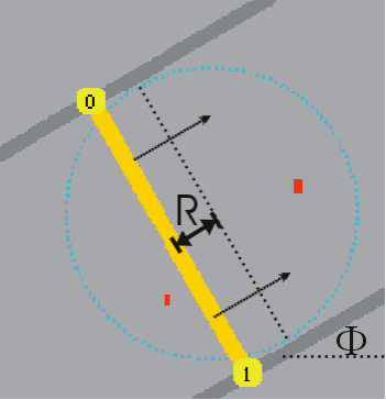
The two detectors (labeled 0 and 1 in fig. 1) are facing each other and can simultaneously move along the gray lines perpendicular to the yellow line connecting the two detectors. This is needed to determine location of the radioactive sources (represented by the red squares) within the blue circle. The gray lines are at an angle with respect to the horizontal. The scan of the two detectors along the grey line is carried out for several different angles. The position of the detectors along the grey line is given by R, the distance from the center of the blue circle and the yellow line connecting the detectors. R can take negative values to distinguish between areas on both sides of the centerline. In fig. 1 R has a negative value. In the simulation we only consider two dimensions.
In the simulation a number of parameters can be set:
- the number of sources and their positions
- the intensity and size of the source(s)
- the detector width and step size for moving the detectors along the grey line (at each step the detectors will check whether (a part of) a source can be seen)
- a start, end and step size for the angle to be used in the scan
The location of one radioactive source
First we we conduct a simulation with only one source present.
Using the button Set sources (see fig. 2), resulting in a second dialog window, allows you to set the positions, intensities and sizes of sources. When you start-up the program this dialog window will automatically be shown.
Location of two radioactive sources
We will investigate what happens when two sources are present.
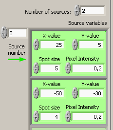
Click on Set sources, set Number of sources to 2 and create a second
source: x = -50, y = -30, spot size 4 and pixel intensity 0.2. Click OK
and remove graphs using RESET All. Take single scans at 0 and 90 degrees. You will observe double peaks in both parallel projections on the left below. Right on top two bars appear at scans for each angle.
When you have completed the scans, you will have four spots where the sources can be located. A scan at a third angle is needed to find the exact location of the sources. Scan at a third angle and check whether you can find the exact location of the sources.
Looking back, would you choose different angles to determine the position of the two sources?
Location of three radioactive sources
Add a third source. Choose any location you like as long as it is within the blue circle. Think about how many angles you should scan at least to locate all three sources. Choose appropriate angles and check whether you can indeed locate the sources.
Figure 1: The PET setup for the simulation. For detail see text above.
Figure 2: The dialog window of the PET simulation
Set a source at the following position: x = 25, y = 5, with a spot size of 5 and a (pixel) intensity of 0.2. The position (with respect to the center of the blue circle) and sizes are given in pixels. Click OK when values are set. Fig. 2 will now show the blue circle with the source in it given by the red square.
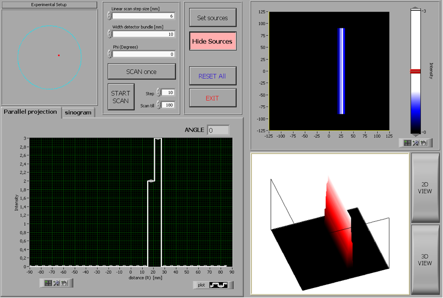
Set the angle at 0 degrees and keep the default settings for the 'Linear scan step size' (6 mm) and 'Width detector bundle' (10 mm) and press SCAN once.
The following will happen:
- Left on top you will see both detectors move along the horizontal.
- On the left below a graph will be plotted of the intensity recorded by the detectors as a function of distance R. When the yellow connecting line passes through the source radiation will be detected. The graph formed is called a parallel projection. It is a projection since all sources on the yellow line between both detectors contribute to the detector signal. No distiction is made with regard of the position of the source on the line. It is a parallel projection because the scan is build up from measurements parallel to each other at different distances R from the center, but under the same angle (in this case 0 degrees).
- Right on top a vertical bar appears. From the scan it follows that the radiactive source is located within this area. The width of this bar is determined by the width of the detectors. This bar is called the Line of Response (LOR). In three dimensions it is called the Tube of Response (TOR). Since from the data taken you do not know where the source is located the intensity measured is distriburted evenly across the bar. Using the slider the color of the intensity distribution can be adjusted (white representing a high intensity, blue a low intensity).
- Right at the bottom you can choose between a 2D and 3D view of the measurement. The graph can be rotated by pressing the left mouse button while moving the cursor.
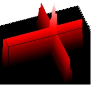
Now set the angle to 90 degrees and press SCAN once again. The detectors will now move along the vertical. On the left below a new intensity graph is added to the first one. Right on top a horizontal bar is added crossing the vertical one. The program calculates for each 2D coordinate the sum of the intensities of the LORs passing through the coordinate. This is also shown below in the 3D graph (see fig. 3).
Figure 3: 3D-view of two projections at 90 degrees for a single source
You have seen that moving the detectors allows measuring signals in a number of positions. This results in a (small) bar, which provides boundaries for the location of the radioactive source. The source can be located more precisely by turning the detectors and taking a second scan, resulting in a second bar. Where the bars cross the source is located. If you know there is only one source, scans at two angles is sufficient to locate it.
Figure 4: Dialog window at Set Sources.
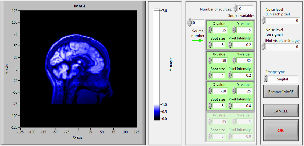
Location of three radioactive sources in the head of a person
So far we have looked at radioactive sources positioned on a dark background. When put in a head it becomes harder to locate them. As explained in the video radioactively labeled sugars are used as a source, which is added to the blood stream. Tumors tend to take up high concentrations of these sugars, but also other tissues will take up sugars. If we consider a human brain with tumors a PET scan will result in an image that shows the brain with more intense spots respresenting the tumors with a high concentration of radioactively labeled sugars. How well they will appear in the image depends on the size of the tumors. To illustrate that detection will become more difficult we will consider three sources in the simulation with the image of the human brain superimposed on it.
Set the sources and image as shown in fig. 5. Take a scan from 0 to 180 degrees with a step size of 10 degrees. Check whether you can find the 3 sources. If not, change the Linear scan step size to 3 mm, Width of detector bundle to 5 mm, Angle step to 2 degrees and Scan till 360 degrees. Can you do it now?
Figure 5: Dialog window for Set sources. The three radioactive sources and the Sagital image should be set.
You failed! Even with the lager number of data gathered it is not possible to reconstract the image directly and located the three radioactive sources. In order to do so, some futher manipulation of data is required. Before we do so, we will first have a look at image processing techniques.
Location of unknown number of radioactive sources
In a real situation you do not know the number of radioactive sources present. In a real situation radioactively labeled sugars are given to a patient through an IV. These sugars accummulate in cancer tissue. The aim of a PET scan is to locate all tumors and their sizes by locating all the radioactive sources and their sizes.
In order to do so you need to perform scans at many different angles. In the simulation you do not need to enter manually. You can enter start and end values and a step size.
Define three sources (e.g. the two you used before and the third one at x = -10, y = 25, spot size 6, intensity 0.4). Set the angle start and end values at 0 and 360 degrees with a step size of 10 degrees. Press START SCAN en follow the build-up of the graphs. During the scan you can switch between 2D- and 3D-View. On the right top window use the slider to show the sources clearly (note: this can only be done after the scans are completed).
Note: if you depress on Draw graphs the simulation will run faster (handy when you take small step sizes).
On the left below you can also switch to the tab sinogram. In a sinogram the scanning angle is plotted against R using different colors to distinguish intensities. It so happens that the position of a source in this coordinate system follows a sine-wave, hence the name sinogram. For further details follow this link. In literature about PET image processing techniques the term sinogram is often used.
When the scans are completed check whether the three sources have been located well (both location and size). At the right on top you can click in the window to enlagre. The Zoom and Hand icon on the right corner can be used to further zoom in or out and to move the graph around in the window.
You can play around a bit with different sizes, locations and intensities of sources. You can also adjust the linear scan step size and the width of the detector bundle. It is important here to realize how these parameters determine how well (accurate) sources can be located (locations and sizes).
In a real PET scanner all scans are taken at once: it has tens of thousands of detectors located in a ring as you have seen in the video at the start.