PET image processing

Simple back projection

A brief introduction to PET image processing will be introduced here. The mathematical tools which are applied are fairly complicated and will not be covered here. We will try to discuss the effects of these mathematical tool on image procesing.

Back projection is the simplest tool, and in the simulation performed so far, this technique has been applied. When two detectors facing each other measure an activity the only thing you can say about it is that the source causing it is located somwhere on the LOR, whose dimensions are determined by the width of the detectors (assuming the linear step size is less than the width of the detectors). Therefore, the most honest way to deal with the data is to distribute the activity evenly accross the LOR.
When a scan is mad at a second angle, another LOR is filled with data. At locations where the LORs cross the activity of both LORs are added.

This process has a big disadvantage: is appears now that there is an activity in regions where there is none in reality. Evenly distributing activity across the LORs comes at a price!

Another consequence is that the closer to a radioactive source, the stronger the activity in the back projection gets. This is due to the fact that near the source the LORs at different angles get closer to each other increasing the chance they will overlap.
This effect is known as 1/r-blurring (blurring that decreases with 1/r, with r the distance to the source). Details about 1/r-blurring can be found here.
If you want to check that this effect does occur repeat a complete scan for one source and carefully determine its size and location.

Fortunately, the above mentioned disadvantages can be reduced substantially using a technique called filtered back projection.

• Simple back projection
• Filtered back projection
• Exercises
• To beginning

Filtered back projection

Filtered back projection corrects the over-representation of activity near the source (the 1/r-blurring).

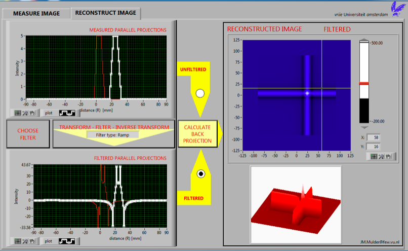
This is done by applying Fourier transfom techniques to individual parallel projections and is called filtering. The effect of it is shown in fig. 1. The filtered parallel projection has a much weaker intensity compared to the original projection and has negative values directly outside the location of the projection of the source. For the filtered projections the positive and negative peaks can be located at different places. Adding all filtered projections result in compensation of wrongfully attributed activity outside the actual sources through the negative values of filtered projections. The result is a much better distribution of activity near the actual location of sources, with much sharper peaks after a back projection.

To illustrate this in the simulation choose one source and scan with a linear scan step of 1 at 0 and 90 degree angles. Select the RECONSTRUCTION IMAGE tab. Click on CHOOSE FILTER, select the Ramp filter, and click on OK (see fig. 1). Next click on the radio button FILTERED, followed by clicking on CALCULATE BACK PROJECTION. The lower graph on the left of fig. 2 shows the filtered parallel projections and the reconstructed image on the right top shows the effect of filtering. The LORs have black liines on the outside, which represent negative intensity values. These negative values compensate for overvalued intensity values along the two LORs where in reality no sources are located. The negative intensity values can also be seen in the lower graph on the right, especially when tilted and slightly rotated (in fig. 2 this was done). From that graph it is clear that the negative intensity values overcompensate near the source. However, when scanning at many angles is undertaken positive overcompensation of intensity values near the source will occur, so this overcompensation of negative intensity values happens to be a good thing. Check this for yourself by conducting a complete scan from 0 to 360 degrees with a step size of 2 degrees.
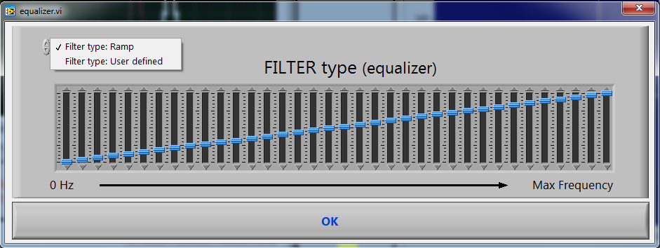
Note that you can also define your own filter. In most cases the ramp filter works well. But do feel free to manipulate the sliders shown in fig. 1 to define your own filter and study its effects.

^Top

^Top

^Top

^Top

Figure 1: Dialog window for selecting the filter type. The Ramp-filter works well in nearly all cases but you can also test out a user defined filter by adjusting the sliders manually.

Figure 2: Filtered image reconstruction from two measured parallel projections

Exercises

A few exercises are presented below to get trained in PET image processing, which is required to succesfully analyse the PET scans collected in the remote lab.

Exercise 1
Define two sources close to each other with (x; y; spot size; intensity) = (25; 5; 5; 0.2) and (34; 5; 5; 0.1).
Scan fro 0 to 180 degrees in setps of 10 degrees with a linear scan step size of 3 mm and a detector width of 5 mm. Check out the image reconstruction with and without filtering (hint: use the zoom and cursor tool on the reconstructed image and the 3D graph to study the effects in detail).

Background radiation
In a real experiment you also need to deal with background radiation due to natural sources. It may also happen that two detectors facing each other accidentally measure a (nearly) signal simultaneously (an accidental coincidence). When you click Set sources you can add a background signal (noise). There are two options:

• Noise level (on each pixel): when you set this to a value, e.g. 3, the program adds to each pixel an intensity between 0 and 3 randomly, thereby simulating a background activity.
• Noise level (on signal): when you set this to a value, e.g. 3, the program adds randomly accidental coincidences with an intensity between 0 and 3.

Exercise 2
Add a background signal to each pixel and define again two sources close to each other, one weak compared to the other. Check how well the sources can be distinguished. Study how this depends on the background signal, the (relative) strength of the sources, the angle step size, etcetera.

Exercise 3
Check how the background that remains left and right of a source of a filtered image depends on the step size of the linear scan and angle scan. Does the detector width effect the results?

Exercise 4
Before we tried to locate sources a head without filtering, and failed to do so. Repeat this exercise again, now including filtering techniques. Start with one source only and find out under which conditions you are able to locate the source. Then add background radiation and accidental coincidences. Determine the minimum sice of a source you can detect and list down under what conditions. When you covered this, try and see if you can detect multiple sources. This may help you understand why in a real PET scanner tens of thousands of detectors are used!