Schrodinger had discovered the equation, named after him, that describes the structure of matter.
It is a differential equation that determines the time evolution of the Hamiltonian representing
a physical system.
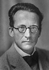 E. Schrodinger
Nobel Prize laureate 1933
E. Schrodinger
Nobel Prize laureate 1933
Although it is not an easy task the Schrodinger equation of the hydrogen atom can be
rogorously solved, following the steps described below.
 The first step in dealing with the time-dependent Schrodinger equation is the one
towards deriving a time-independent equation. If the potential function
V(x,y,z,t) is independent of the time-coordinate, and can be written as
V(x,y,z), it can be shown that the wave function can be separated in a
spatial part and a temporal part.
The latter is an oscillatory function of time. The spatial part of the wave function then obeys the
time-independent Schrodinger equation.
The first step in dealing with the time-dependent Schrodinger equation is the one
towards deriving a time-independent equation. If the potential function
V(x,y,z,t) is independent of the time-coordinate, and can be written as
V(x,y,z), it can be shown that the wave function can be separated in a
spatial part and a temporal part.
The latter is an oscillatory function of time. The spatial part of the wave function then obeys the
time-independent Schrodinger equation.
Proof
In principle the Hamiltonian is based on 6 coordinates, 3 for each particle. The system can
be transformed to the centre-of-mass frame with relative coordinates (x,y,z)
and the coordinates (X,Y,Z) describing the kinetic motion of the entire system.
This transformation results in replacing the mass of the electron m by its reduced
mass mu, in fact only a change with small effect.
Proof (pdf)
The time-independent Schrodinger equation is then transformed from a Cartesian basis
(x,y,z) to a basis of
spherical polar coordinates (r, theta, phi). Note that a Jacobian has to be
calculated, to be used in all integrals over a volume element.
Since the Coulomb potential in the two-particle system of the hydrogen atom is only a
function of the interparticle separation this procedure will be helpful in finding
solutions.
Proof
The resulting time-independent Schrodinger equation in spherical coordinates, with a
potential dependent on only one coordinate V(r), is a partial differential
equation that can however be separated into three different ordinary
differential equations.
here.
Math: separation of variables.
Then the three differential equations can be solved each at a time. All three
involve a quantization condition, that results from the mathematics of solving
the equation: only solutions are found for some integer parameters, which we
call quantum numbers. Since there are three differential equations, there are
three quantum numbers
that describe the physical system of the hydrogen atom.
Note that the first step of separation the time coordinate also gave a parameter,
which is the energy of the quantum state. This energy only plays a role in the differential equation
for the coordinate r, so in the radial equation. This has as the important consequence for
the hydrogen atom, that only the quantum number n, associated with the radial part,
is energy dependent.
The solutions of the angular part is NOT dependent on the energy; that is the reason
why the energy levels of the hydrogen atom do not depend on quantum numbers l and m.
So the energy levels are degenerate in l and m !
Each of the three wave equations gives a solution in terms of a wave function.
The angular part results in the so-called
spherical harmonic functions.
These three-dimensional functions can be plotted in
2D-pictures.
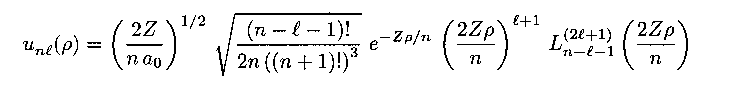
The radial equation results in complicated functions known as the
Laguerre polynomials:
These functions
can be multplied to yield the total wave function of the system (multiplication
of the time-dependent oscillatory part should also be done).
The general equations for arbitrary quantum numbers have complicated expressions,
but for the lowest quantum numbers the mathematical expressions for
wave functions look relatively simple.
This treatment of the Schrodinger equation yields the Rydberg formula for the
energy levels
and thus provides the Bohr model with a consistent physical basis.
So also the transitions wavelengths and
the
spectrum of the hydrogen atom
can now be fundamentally understood.
Analysis of the radial wave functions can be performed by
plotting these functions
along the radial coordinate, thus given insight in the extension of the
electronic structure of the system, not only for the ground state but
also for the electronically excited states.
With the use of the quantum mechanical definition of expectation value the
most probable radius
of the ground state can be shown to equal the Bohr radius a0.
Furthermore average values of the radial distribution can be calculated in
terms of
expectation values.
An important property of the wave function is its parity. This property of
quantum mechanical wave functions is in the case of the hydrogen atom
entirely determined by the spherical harmonics angular functions.
It can be easily verified
(click here) that the parity of a wave function follows the simple rule:
- states of even l quantum number have even parity
- states with odd values of l have odd parity.
 Note that there are other coordinate frames in which the Schrodinger equation for
the hydrogen atom is separable. One example is that of parabolic coordinates,
useful for the evaluation of the
Stark effect.
Note that there are other coordinate frames in which the Schrodinger equation for
the hydrogen atom is separable. One example is that of parabolic coordinates,
useful for the evaluation of the
Stark effect.
Math: Separation of variables in parabolic coordinates.
The treatment of the hydrogen atom in the framework of the Schrodinger equation
yields understanding of two important issues related to the quantum states:
 The wave functions, calculated in three dimensions, represent an electron density
in the atom. This is usually referred to as the "atomic orbitals" or as "electron clouds".
It should however be noted that the orbitals do
NOT represent a spatial distribution of electronic
density at a certain moment in time, an idea initally conceived by Schrodinger. This
concept leads to contradictions in the physical picture. The "electron cloud"
should be interpreted according to the ideas of Born: it represents a
probability
that the electron is found at a certain point in space
in the atom.
In principle this probability distribution can be time-dependent
(
for superposition states);
for stationary states this is not the case.
The wave functions, calculated in three dimensions, represent an electron density
in the atom. This is usually referred to as the "atomic orbitals" or as "electron clouds".
It should however be noted that the orbitals do
NOT represent a spatial distribution of electronic
density at a certain moment in time, an idea initally conceived by Schrodinger. This
concept leads to contradictions in the physical picture. The "electron cloud"
should be interpreted according to the ideas of Born: it represents a
probability
that the electron is found at a certain point in space
in the atom.
In principle this probability distribution can be time-dependent
(
for superposition states);
for stationary states this is not the case.
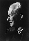 Max Born
Nobel Prize laureate 1954
Max Born
Nobel Prize laureate 1954
Here some orbitals are shown, in a 2D projection of 3D pictures:
 1s0
1s0
 3d1
3d1
 9i3
9i3
 10p0
10p0
 4s0
4s0
 4f2
4f2
The three digit arguments represent:
- the value of n;
- the value of l; s for l=0, p for l=1, d for l=2, f for l=3, g for l=4, etc.
- the value of m; this is defined only with respect to a defined z-axis.
This is in line with conventions on
the spectroscopic notation of the orbitals.
An overview of a large number of atomic orbitals can be found
here.
In classical electrodynamics radiation is a result of accelerated charges, such as the
oscillation of an electric dipole.
In quantum mechanics there are stationary states between which transitions can occur
through "quantum jumps". By analogy to the classical theory a "transition dipole moment"
is defined in quantum mechanics.
The transition amplitude is equal to the operator er sandwitched
between two quantum states:
< Psii|er|Psif>.
In fact the
expectation value of the dipole operator is calculated.
This gives a quantummechanical theory for the intensity of spectral lines !
Note that:
This treatment applied to one
and the same state yields a value of zero, since atoms do not have a
permanent dipole moment; atoms only have a transition dipole moment.
In quantum mechanics, as well as in classical theory, higher order multipole moments
can give rise to transitions, but these are much weaker; for atoms the electric quadrupole
or magnetic dipole transitions are generally 6 orders of magnitude weaker.
In nuclear physics however they are not so much weaker.
The mathematical representation of the transition amplitude not only gives the intensities
as such, but it allows us to deduce general rules for which transitions are allowed
and which are forbidden. Selection rules can be derived which can be expressed as
relations between quantum numbers of ground |nlm> and excited |n'l'm'> states.
Math: Selection Rules:
n: no rule; all is possible
l: change in l = +/- 1
m: change in m = 0 (for linearly polarized light), = +1
(for right-handed circularly polarized light),
= -1 (for left-handed circularly polarized light).
Some advanced topics on the spectrum of the hydrogen atom
 Last change: 1 November 2001
E. Schrodinger
Nobel Prize laureate 1933
The first step in dealing with the time-dependent Schrodinger equation is the one
towards deriving a time-independent equation. If the potential function
V(x,y,z,t) is independent of the time-coordinate, and can be written as
V(x,y,z), it can be shown that the wave function can be separated in a
spatial part and a temporal part.
The latter is an oscillatory function of time. The spatial part of the wave function then obeys the
time-independent Schrodinger equation.Proof
In principle the Hamiltonian is based on 6 coordinates, 3 for each particle. The system can
be transformed to the centre-of-mass frame with relative coordinates (x,y,z)
and the coordinates (X,Y,Z) describing the kinetic motion of the entire system.
This transformation results in replacing the mass of the electron m by its reduced
mass mu, in fact only a change with small effect.Proof (pdf)
The time-independent Schrodinger equation is then transformed from a Cartesian basis
(x,y,z) to a basis of
spherical polar coordinates (r, theta, phi). Note that a Jacobian has to be
calculated, to be used in all integrals over a volume element.
Since the Coulomb potential in the two-particle system of the hydrogen atom is only a
function of the interparticle separation this procedure will be helpful in finding
solutions.Proof
The resulting time-independent Schrodinger equation in spherical coordinates, with a
potential dependent on only one coordinate V(r), is a partial differential
equation that can however be separated into three different ordinary
differential equations.here. Math: separation of variables.
Then the three differential equations can be solved each at a time. All three involve a quantization condition, that results from the mathematics of solving the equation: only solutions are found for some integer parameters, which we call quantum numbers. Since there are three differential equations, there are three quantum numbers that describe the physical system of the hydrogen atom. Note that the first step of separation the time coordinate also gave a parameter, which is the energy of the quantum state. This energy only plays a role in the differential equation for the coordinate r, so in the radial equation. This has as the important consequence for the hydrogen atom, that only the quantum number n, associated with the radial part, is energy dependent. The solutions of the angular part is NOT dependent on the energy; that is the reason why the energy levels of the hydrogen atom do not depend on quantum numbers l and m. So the energy levels are degenerate in l and m !
Each of the three wave equations gives a solution in terms of a wave function.
The angular part results in the so-called
spherical harmonic functions.
These three-dimensional functions can be plotted in
2D-pictures.
The radial equation results in complicated functions known as the Laguerre polynomials:
These functions can be multplied to yield the total wave function of the system (multiplication of the time-dependent oscillatory part should also be done). The general equations for arbitrary quantum numbers have complicated expressions, but for the lowest quantum numbers the mathematical expressions for wave functions look relatively simple.
This treatment of the Schrodinger equation yields the Rydberg formula for the
energy levels
and thus provides the Bohr model with a consistent physical basis.
So also the transitions wavelengths and
the
spectrum of the hydrogen atom
can now be fundamentally understood.
Analysis of the radial wave functions can be performed by
plotting these functions
along the radial coordinate, thus given insight in the extension of the
electronic structure of the system, not only for the ground state but
also for the electronically excited states.
With the use of the quantum mechanical definition of expectation value the
most probable radius
of the ground state can be shown to equal the Bohr radius a0.Furthermore average values of the radial distribution can be calculated in terms of expectation values.
An important property of the wave function is its parity. This property of
quantum mechanical wave functions is in the case of the hydrogen atom
entirely determined by the spherical harmonics angular functions.
It can be easily verified
(click here) that the parity of a wave function follows the simple rule:- states of even l quantum number have even parity
- states with odd values of l have odd parity.
Note that there are other coordinate frames in which the Schrodinger equation for
the hydrogen atom is separable. One example is that of parabolic coordinates,
useful for the evaluation of the
Stark effect.Math: Separation of variables in parabolic coordinates.
The wave functions, calculated in three dimensions, represent an electron density
in the atom. This is usually referred to as the "atomic orbitals" or as "electron clouds".
It should however be noted that the orbitals do
NOT represent a spatial distribution of electronic
density at a certain moment in time, an idea initally conceived by Schrodinger. This
concept leads to contradictions in the physical picture. The "electron cloud"
should be interpreted according to the ideas of Born: it represents a
probability
that the electron is found at a certain point in space
in the atom.
In principle this probability distribution can be time-dependent
(
for superposition states);
for stationary states this is not the case.
Max Born
Nobel Prize laureate 1954Here some orbitals are shown, in a 2D projection of 3D pictures:
1s0
3d1
9i3
10p0
4s0
4f2
The three digit arguments represent:
- the value of n;
- the value of l; s for l=0, p for l=1, d for l=2, f for l=3, g for l=4, etc.
- the value of m; this is defined only with respect to a defined z-axis.
This is in line with conventions on the spectroscopic notation of the orbitals.
An overview of a large number of atomic orbitals can be found here.
In classical electrodynamics radiation is a result of accelerated charges, such as the
oscillation of an electric dipole.In quantum mechanics there are stationary states between which transitions can occur through "quantum jumps". By analogy to the classical theory a "transition dipole moment" is defined in quantum mechanics. The transition amplitude is equal to the operator er sandwitched between two quantum states: < Psii|er|Psif>.
In fact the expectation value of the dipole operator is calculated.
This gives a quantummechanical theory for the intensity of spectral lines !
Note that:
This treatment applied to one
and the same state yields a value of zero, since atoms do not have a
permanent dipole moment; atoms only have a transition dipole moment.
In quantum mechanics, as well as in classical theory, higher order multipole moments
can give rise to transitions, but these are much weaker; for atoms the electric quadrupole
or magnetic dipole transitions are generally 6 orders of magnitude weaker.
In nuclear physics however they are not so much weaker.
The mathematical representation of the transition amplitude not only gives the intensities
as such, but it allows us to deduce general rules for which transitions are allowed
and which are forbidden. Selection rules can be derived which can be expressed as
relations between quantum numbers of ground |nlm> and excited |n'l'm'> states.Math: Selection Rules:
n: no rule; all is possible
l: change in l = +/- 1
m: change in m = 0 (for linearly polarized light), = +1
(for right-handed circularly polarized light),
= -1 (for left-handed circularly polarized light).