Atomic Physics
1. Historical perspective
In the years before Bohr formulated his theory of the atom, based upon the principles
of quantum physics, some steps had been made on the understanding of the
atomic structure. We list here some important contributions:
 Mendeleev had developed a concept for arranging the known chemical elements based on their mass.
Order was given in terms of increasing mass, while the elements were further arranged according
to the ordering principle of chemical behaviour.
The columns in the table of the elements relate to chemical valence. In 1869 the
Periodic Table
was not yet complete.
Mendeleev had developed a concept for arranging the known chemical elements based on their mass.
Order was given in terms of increasing mass, while the elements were further arranged according
to the ordering principle of chemical behaviour.
The columns in the table of the elements relate to chemical valence. In 1869 the
Periodic Table
was not yet complete.
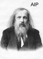 D.I. Mendeleev
Avogadro had conceived the idea that gasses consist of discrete particles and had established
the law that equal volumes of gas at equal pressure and temperature contain the SAME number
of such particles, although the actual number was not yet determined.
Avogadro's hypothesis was not accepted by many physicists for a long time.
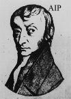 A. Avogadro.
The work on the analysis of the "Brownian motion" turned out to be decisive for the acceptance
of the particle hypothesis. First the botanist Brown had looked at grains of pollen moving in a
liquid through observation by a microscope. Then Einstein developed his theory of the Brownian
motion based on the ideas of diffusion and random walk.
Look here for Brownian motion
in action.
As a final outcome Einstein deduced the
important relation between the Boltzman constant kB and the universal gas constant R:
kB = R/NA
where NA is Avogadros number. This lead J.B. Perrin to a measurement of this important value
yielding:
NA = 6.0221 x 10²³ molecules/mole, which is not far off from the true value.
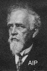 J.B. Perrin
Nobel Prize laureate 1926
J.B. Perrin
Nobel Prize laureate 1926
It was realized for some time that electrostatic charges were important for the building blocks
of matter. This followed from Faradays experiments on
electrolysis
, from which it was deduced that
ions move in a liquid as charged particles, and from the experiments on radioactivity in which
electrically charged particles were emitted.
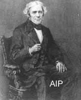 M. Faraday
Thomson's experiments on cathode rays were important for the determination of some properties
of the constituents of matter. The charged particles, emitted from a cathode, were deflected in
a combination of crossed static electric and magnetic fields,
and detected on the phosphorent screen (see Fig). Hence impinging
charged particles could be made visible by the light emitted by the screen.
The experiment is based upon an
analysis of the kinematics of the particles, deflected by a field
as explained
here.
A value can be determined for the e/m ratio:
e/m = 1.75 x 10¹¹ C/kg.
for the small charged particle which was named the "electron". The
electron was discovered (as an elementary particle) in 1897.
 J.J. Thomson
Nobel Prize laureate 1906
J.J. Thomson
Nobel Prize laureate 1906
The results on cathode rays and their interpretation,
sometimes referred to as "
mysterious rays", were long
debated among scientists
(
click here).
After the ratio (e/m) was determined Millikan performed his famous
oil-drop experiment
from which the two values of e and m could be unravelled. In fact Millikan also
proved the discreteness of charge in his experiment of 1906.
 R.A. Millikan
Nobel Prize laureate 1923
R.A. Millikan
Nobel Prize laureate 1923
Based on these concepts Thomson developed a model for the atom consisting of the electrons
as negatively charged particles of low mass and some substance that should carry positive
charge and nearly all the mass within the atom. Since the elements were arranged according
to their mass nemuber A, the atoms were thought to consist of A positive particles and A electrons
in a structure as shown below.
Note that the atomic number Z does not play a role yet.
Atomic Models
 Thomson's model
 Rutherford's model
After his studies into radioactivity Rutherford set out, in the first decade of the
20th century, to perform
scattering experiments with alpha-particles, to investigate
the structure of the atom.
A full theoretical treatment on the physical concepts and scattering cross sections
can be found
here.
Two important conclusions could be drawn from the
angular distribution of the scattered particles:
- almost all the particles were transmitted through a foil of metal without any deflection
- a very few particles were scattered backwards into the detector
From detailed analyses of the scattering kinematics of charged particles (known as
Rutherford scattering) it was concluded that the atom consists of:
 merely a void
with a heavy positively charged nucleus at the centre carrying all the mass of the atom
within a size of a few fm (10-15 m)
electrons outside the nucleus
 E. Rutherford
Nobel Prize laureate 1908 (Chemistry)
E. Rutherford
Nobel Prize laureate 1908 (Chemistry)
There are however a number of shortcomings to this planetary model of an atom bound by
classical electromagnetic forces:
 the problem of stability with accelerated electrons in orbit loosing energy
the model gives no indication of the size of the atom
the model gives no explanation for the characteristic spectroscopy of atoms
All these contributions, mentioned above,
lead jointly to a conception of the structure of atoms. There is
however another branch of research that has in the past, and as of today, taught us most
about the structure of atoms and molecules.
2. Spectroscopy
Spectroscopy, or the physics of the interaction between light and matter, with an emphasis
of the wavelength dependences, is a field of research that yields extremely accurate
information. This is because wavelength, or rather frequency, is the quantity that can be
measured most accurately. Spectroscopy was initially closely connected to the
development of optical instruments used for the dispersion of light into its wavelength
components. The prism and the grating were the instruments developed for this purpose.
Later the field of spectroscopy became closely connected to that of the laser.
Investigations of atomic spectra began in the 19th century with the work of
J. von Fraunhofer,
who measured and interpreted the spectrum of the sun. The lines, that have over the years been
studied in high precision (see
Table), originate from atoms (and ions) in the sun and from absorbers in the Earth's atmosphere.
Fraunhofer spectrum of the sun
Kirchhoff
explained the difference between
absorption and emission spectra. Moreover he showed that each observed spectrum was
characteristic for the chemical species that is interacting with the light. This made it
possible to identify new elements, such as cesium and
rubidium, based on spectroscopic
observations.
The element helium, for the Greek helios, or Sun, was first
discovered in 1868 in the spectra of solar flares,
using the techniques of Bunsen and Kirchhoff, before it was shown to exist on Earth,
also from its spectrum.
The characteristic
yellow resonance line
in helium is very close to the
doublet of sodium.
The Scottish chemist
William Ramsay heated the mineral cleveite, and found small traces of the element helium
much later in 1895.
As of today an enormous amount of spectroscopic work has been
performed, that is carefully listed for the scientific community in accesible databases.
Such databases exist for observed
line spectra in the form of tabulations of lines pertaining to
a certain element, but also to the charge state of the species.
The species are, e.g. for iron, identified as Fe I for the neutral iron atom,
Fe II for the singly ionized iron,
Fe III for the doubly ionized iron or Fe++, etc.
Such spectra were already collected in the 19th century, but since no
ordering principle was available at that time, they were like stamp collections.
Balmer
was the first to recognize a regularity in a series of lines of the hydrogen atom
as early as 1885. The visible lines could be fitted to the formula for the
Balmer series:
L = LA n2/(n2 - 4) for n>2
yielding a constant LA = 364.56 nm.
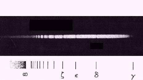
Balmer series observed in a hot A-type star
Later in 1890
Rydberg
generalized the series treatment by including other progressions of lines in
the hydrogen atom yielding the equation:
1/L = RH (1/n2 - 1/m2)
for integer n and m and the constant RH = 10972160 m-1,
which was named the
Rydberg constant.
 J. Rydberg
Balmer's series fits to n=2, while the predicted n=3 series
was observed by Paschen in 1908.
The latter was possible by opening up the infrared region of the
electromagnetic spectrum for spectroscopy.
At the other end, the domain of the vacuum ultraviolet
(at wavelengths shorter than 200 nm, where the atmosphere does not
transmit the light and vacuum techniques have to be employed)
Schumann performed pioneering studies and Lyman
recorded the n=1 series of the H-atom in 1914. The understanding of the line
structure remained limited to the hydrogen atom, and even there,
a deeper insight into the origin of the Rydberg regularity was lacking.
3. The Bohr model of the atom
Rutherford's planetary model of the atom was understood
in terms of classical electrodynamics. This model could in principle
explain the occurrence of radiation, since in Maxwell's theory,
light is emitted by accelerated charges, hence by the electrons in orbit.
(Note that acceleration is required in a circular orbit)
At the same time this causes a contradiction in the theory,
since the decelerated electrons, while emitting light, would continuously
loose energy, collaps with the nucleus and make the atoms unstable.
So the quest was for a theory explaining the stability of the atom
and the existence of stationary states.
Bohr made a break with classical physics by adopting notions from quantum
theory and by simply postulating the existence of stationary states.
The assumptions of Bohr were simply:
 the electron is in a stationary state of which there exist a discrete set
a quantisation condition is given by: L = nh, where L is the angular momentum of the eletron,
n is a positive integer and h is
Planck's constant.
transitions between these states are possible with frequency v, v given by:
hv = Em - En
 N. Bohr
Nobel Prize laureate 1922
N. Bohr
Nobel Prize laureate 1922
Within this model Bohr could give a
Mathematical derivation of the Rydberg formula.
A few comments on Bohr's model:
the quantisation condition is introduced in an ad hoc way without a justification
an explanation is given for the frequencies of the observed optical transitions (spectra)
but a theory of radiative transitions is still lacking
an explanation for the intensities of the spectral lines is not yet given
the Bohr model does give us a theory for the size of the atom
the model works only for the hydrogen atom;
spectra of other atoms are not yet explained
Extension of the Bohr-model
Bohr, in his semiclassical analysis, had only allowed for circular orbits in his model.
Later the model was extended by
Sommerfeld also allowing for elliptical orbits.
This version, based on the same ad hoc quantization condition for the
angular momentum is referred to as the
Bohr-Sommerfeld model.
Sommerfeld already postulated the azimuthal quantum number,
in addition to the principle quantum number n defined by Bohr.
Explanation of characteristic X-rays in the Bohr-model
Based on the Bohr model also the observed characteristic X-rays of more than 40
elements could be explained. Moseley performed a
comprehensive study of the X-rays
and their characteric wavelengths.
The
characteristic X-rays with a typical resonance structure,
should be distinguished from background X-rays, known as "Bremsstrahlung".
An interesting aspect of this work is that the characteristic frequency of some
K or L lines can be
plotted as a function of the element with the
atomic number Z on one axis.
A
derivation shows the Z vs root-frequency law for characteristic
X-rays.
The K and L indices refer to the shell to where the atoms decay to the
X-ray transition.
This method hence allows for an identification of
the atomic number Z by experimental means. So the periodic system could finally
be given in terms of Z instead of the mass number, and even some questionable
assignements of elements could be resolved.
4. The Schrodinger equation of the hydrogen atom
Schrodinger had discovered the equation, named after him, that describes the structure of matter.
It is a differential equation that determines the time evolution of the Hamiltonian representing
a physical system.
Although it is not an easy task the Schrodinger equation of the hydrogen atom can be
rogorously solved, following the steps described below.
The first step in dealing with the time-dependent Schrodinger equation is the one
towards deriving a time-independent equation. If the potential function
V(x,y,z,t) is independent of the time-coordinate, and can be written as
V(x,y,z), it can be shown that the wave function can be separated in a
spatial part and a temporal part.
The latter is an oscillatory function of time. The spatial part of the wave function then obeys the
time-independent Schrodinger equation.
Proof
In principle the Hamiltonian is based on 6 coordinates, 3 for each particle. The system can
be transformed to the centre-of-mass frame with relative coordinates (x,y,z)
and the coordinates (X,Y,Z) describing the kinetic motion of the entire system.
This transformation results in replacing the mass of the electron m by its reduced
mass mu, in fact only a change with small effect.
Proof (pdf)
The time-independent Schrodinger equation is then transformed from a Cartesian basis
(x,y,z) to a basis of
spherical polar coordinates (r, theta, phi). Note that a Jacobian has to be
calculated, to be used in all integrals over a volume element.
Since the Coulomb potential in the two-particle system of the hydrogen atom is only a
function of the interparticle separation this procedure will be helpful in finding
solutions.
Proof
The resulting time-independent Schrodinger equation in spherical coordinates, with a
potential dependent on only one coordinate V(r), is a partial differential
equation that can however be separated into three different ordinary
differential equations.
here.
Math: separation of variables.
Then the three differential equations can be solved each at a time. All three
involve a quantization condition, that results from the mathematics of solving
the equation: only solutions are found for some integer parameters, which we
call quantum numbers. Since there are three differential equations, there are
three quantum numbers
that describe the physical system of the hydrogen atom.
Note that the first step of separation the time coordinate also gave a parameter,
which is the energy of the quantum state. This energy only plays a role in the differential equation
for the coordinate r, so in the radial equation. This has as the important consequence for
the hydrogen atom, that only the quantum number n, associated with the radial part,
is energy dependent.
The solutions of the angular part is NOT dependent on the energy; that is the reason
why the energy levels of the hydrogen atom do not depend on quantum numbers l and m.
So the energy levels are degenerate in l and m !
Each of the three wave equations gives a solution in terms of a wave function.
The angular part results in the so-called
spherical harmonic functions.
The radial equation results in complicated functions known as the
Laguerre polynomials:
 Math: derivation.
These functions
can be multplied to yield the total wave function of the system (multiplication
of the time-dependent oscillatory part should also be done).
The general equations for arbitrary quantum numbers have complicated expressions,
but for the lowest quantum numbers the mathematical expressions for
wave functions look relatively simple.
This treatment of the Schrodinger equation yields the Rydberg formula for the
energy levels
and thus provides the Bohr model with a consistent physical basis.
So also the transitions wavelengths and
the
spectrum of the hydrogen atom
can now be fundamentally understood.
Analysis of the radial wave functions can be performed by
plotting these functions
along the radial coordinate, thus given insight in the extension of the
electronic structure of the system, not only for the ground state but
also for the electronically excited states.
With the use of the quantum mechanical definition of expectation value the
most probable radius
of the ground state can be shown to equal the Bohr radius a0.
Furthermore average values of the radial distribution can be calculated in
terms of
expectation values.
An important property of the wave function is its parity. This property of
quantum mechanical wave functions is in the case of the hydrogen atom
entirely determined by the spherical harmonics angular functions.
It can be easily verified
(click here) that the parity of a wave function follows the simple rule:
- states of even l quantum number have even parity
- states with odd values of l have odd parity.
Note that there are other coordinate frames in which the Schrodinger equation for
the hydrogen atom is separable. One example is that of parabolic coordinates,
useful for the evaluation of the
Stark effect.
Math: Separation of variables in parabolic coordinates.
The treatment of the hydrogen atom in the framework of the Schrodinger equation
yields understanding of two important issues related to the quantum states:
The wave functions, calculated in three dimensions, represent an electron density
in the atom. This is usually referred to as the "atomic orbitals" or as "electron clouds".
It should however be noted that the orbitals do
NOT represent a spatial distribution of electronic
density at a certain moment in time, an idea initally conceived by Schrodinger. This
concept leads to contradictions in the physical picture. The "electron cloud"
should be interpreted according to the ideas of Born: it represents a
probability
that the elctron is found at a certain point in space
in the atom.
In principle this probability distribution can be time-dependent
(
for superposition states);
for stationary states this is not the case.
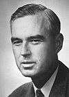
 Max Born
Nobel Prize laureate 1954
Max Born
Nobel Prize laureate 1954
Here some orbitals are shown, in a 2D projection of 3D pictures:
 1s0
1s0
 3d1
3d1
 9i3
9i3
 10p0
10p0
 4s0
4s0
 4f2
4f2
The three digit arguments represent:
- the value of n;
- the value of l; s for l=0, p for l=1, d for l=2, f for l=3, g for l=4, etc.
- the value of m; this is defined only with respect to a defined z-axis.
This is in line with conventions on
the spectroscopic notation of the orbitals.
An overview of a large number of atomic orbitals can be found
here.
In classical electrodynamics radiation is a result of accelerated charges, such as the
oscillation of an electric dipole.
In quantum mechanics there are stationary states between which transitions can occur
through "quantum jumps". By analogy to the classical theory a "transition dipole moment"
is defined in quantum mechanics.
The transition amplitude is equal to the operator er sandwitched
between two quantum states:
< Psii|er|Psif>.
In fact the
expectation value of the dipole operator is calculated.
This gives a quantummechanical theory for the intensity of spectral lines !
Note that:
This treatment applied to one
and the same state yields a value of zero, since atoms do not have a
permanent dipole moment; atoms only have a transition dipole moment.
In quantum mechanics, as well as in classical theory, higher order multipole moments
can give rise to transitions, but these are much weaker; for atoms the electric quadrupole
or magnetic dipole transitions are generally 6 orders of magnitude weaker.
In nuclear physics however they are not so much weaker.
The mathematical representation of the transition amplitude not only gives the intensities
as such, but it allows us to deduce general rules for which transitions are allowed
and which are forbidden. Selection rules can be derived which can be expressed as
relations between quantum numbers of ground |nlm> and excited |n'l'm'> states.
Math: Selection Rules:
n: no rule; all is possible
l: change in l = +/- 1
m: change in m = 0 (for linearly polarized light), = +1
(for right-handed circularly polarized light),
= -1 (for left-handed circularly polarized light).
Some advanced topics on the spectrum of the hydrogen atom
Relativistic effects
The Schrodinger equation, taken as the starting point for this section, is of course
the non-relativistic one. In view of the fact that the characteristic energy in the hydrogen atom,
the Rydberg energy, scales like (alpha)2
(hyperlink to introduction) times the rest-mass,
the electron relativistic effects are small. The kinetic energy operator, which is classically
p2/2m, can relativistically be written in a power series expansion,
with the classical term as the first, added by a term proportional to p4.
Since the wave functions of the Hydrogen atom are eigen functions of the operator
p2, they are also eigenfunctions of the operator p4, so that
the first and higher order relativistic corrections can be easily calculated.
Note that the contribution of relativistic (kinetic) effects
are equally large as the spin-orbit interaction effects in hydrogen.
Math: derivation.
A comprehensive first priciples description of the hydrogen atom from the relativistic
point of view is given in terms of the
Dirac equation, in which automatically
the effects of electron spin are included.
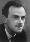 Paul Dirac
Nobel Prize laureate 1933
Paul Dirac
Nobel Prize laureate 1933
Quantum electrodynamics effects and the Lamb shift
Even the relativistic Dirac equation does not give an exact treatment of the hydrogen atom
for the reason that the theory of quantum mechanics should be extended somewhat with the
effects of the self-energy of the electron and the vacuum polarisation. The theory
of Quantum Electrodynamics, developed by Tomonaga, Feynman, and Schwinger, is the theory
superseeding quantum mechanics. It gives the most accurate description of the structure
of matter and includes these effects.
One result of QED is the deviation of the g-factor for the electron from 2.
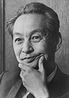

Tomonaga, Feynman and Schwinger
Nobel Prize laureates 1965
One of the effects of QED is the splitting between the 2s and 2p levels in atomic hydrogen,
first observed
by Lamb and Retherford by means of inducing a microwave transition between these levels.
As mentioned, these levels are expected to be degenerate in the framework of the Schrodinger
equation.
From an advanced analysis within QED it can be
shown that the self-energy of the electron, or the electron mass renormalization,
gives the dominant contribution to the Lamb shift of 1060 MHz.
Later the Lamb shift was also observed via the technique of
laser saturation spectroscopy.
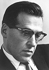
 W.E. Lamb
Nobel Prize laureate 1955
W.E. Lamb
Nobel Prize laureate 1955
Measurements of these small effects in the spectra of atoms has become an active field of
physics. Also at Vrije Universiteit an important contribution has been made in this area
by the measurement of the Lamb shift in the ground state of the
Helium atom.
Hyperfine structure
The nucleus of the hydrogen atom, the proton, has a nuclear spin of IH = 1/2.
The associated magnetic dipole moment interacts with the spin of the electron
via a magnetic coupling, similar to that of the spin-orbit interaction.
This interaction gives rise to a splitting of the ground state of hydrogen
|n=0, l=0, j=1/2> into a F=1 level and a F=0 level,
F being the total angular momentum including the nuclear spin.
It can be shown that the splitting, named the hyperfine splitting, is 1420 MHz.
Calculation of hyperfine structure in hydrogen.
Furthermore it can be calculated that the spontaneous decay rate of the upper F=1 level is
A10 = 3 x 10-15 s-1.
This decay rate corresponds to an upper state lifetime of 107 years.
So this is a very weak transition, related to the fact that an electric dipole transition
between the hyperfine levels is forbidden; both levels have l=0 and therefore the same
parity.
Math: Calculation of decay of F=1 level (difficult).
The transition frequency of 1420 MHz corresponds to a wavelength of 21 cm.
Although the transition probability in a single atom is very weak, the abundance
of H-atoms in the universe is so high that the 21 cm line is a spectral feature that is
readily observable with
radio telescopes. In the Netherlands there has been a strong activity
in radio-astronomy since the 1950's, centered around the observatory in
Westerbork-Dwingelo.
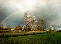 Westerbork-Dwingelo Radiotelescope
In fact
Sky surveys of 21 cm line
can be made, hence mapping out the hydrogen in the universe.
5. Optical transitions in a two-level system
Einstein, in his pivotal paper of 1917, discussed the radiation balance in a
generalized two-level system. Here he postulated the concept of stimulated emission,
in addition to the intuitively understood concepts of absorption and spontaneous
emission.
Involved are two levels, with energies E2 (upper) and E1 (lower)
and populations n2 and n1.
The radiation field at frequency v (monochromatic), with energy density uv
is considered to be resonant with the energy separation:
E2 - E1 = hv.
Picture Einstein model
Einstein defined three processes:
Absorption; this process is proportional to the population of the ground state and the
density of the radiation field uv; a proportionality constant is defined as C.
Spontaneous emission; this process is only proportional to the population of the excited
state and not to a radiation field density;
the proportionality constant is A.
Stimulated emission; maybe counter intuitively, Einstein defined a process of emission
induced by the radiation field; it is proportional to the population density
n2 as some inverse absorption process; the proportionality constant is B.
The three proportionality constants A, B and C are the "Einstein coefficients".
Then rate equations can be written for the population of the states:
dn2/dt = Cuvn1 - (A + Buv)n2
In the steady state condition (dn2/dt = 0) this gives:
n1/n2 = (A + Buv) / Cuv
Now, as a result from statistical phsyics, for the case of thermodynamic
equilibrium at temperature T, the
Maxwell-Boltzman distribution defines the probability
that a level is thermally excited.
Hence:
n1/n2 = exp(-E1/kT) / exp(-E2/kT)
= exp(hv/kT)
where k is the
Boltzmann constant.
When it is now assumed that the (atomic) two-level system is in thermodynamic
equilibrium with its environment at temperature T, the two equations for the
ratio n1/n2 yield an equation for the radiation field
expressed in terms of the Einstein coefficients; this procedure can be
understood as the radiative processes creating the equilibrium:
uv = A / (Cexp(hv/kT) - B)
For radiative balance between a body at temperature T and a radiation field uv
Planck's radiation formula should hold. Indeed the formula for uv
has the structure of Planck's equation.
The derived equation for uv agrees with that of Planck if the following simple
relations between the Einstein coefficients are adopted:
B = C; so stimulated emission is equally "strong" as absorption
A/B = 8(pi)hv3/c3; giving a relation between spontaneous and stimulated
emission
The Einstein B-coefficient, or the strength of an absorption line, should be proportional to the
square of the transition amplitude, i.e. the expectation value of the transition
dipole moment. The exact formula can be derived from a quantummechanical
treatment of the interaction between light and matter. Without proof we give:
Equation for C
The coefficient for spontaneous emission then automatically follows from
the above derivation of the Einstein coefficients:
Equation for A
The above has some interesting physical consequences:
In the absence of a radiation field (uv = 0) the dynamical rate equations reduce
to:
dn2/dt = -An2.
With the boundary condition
n2(0) = N, so initially all population in the excited state, this gives
an exponential decay function, with A as the decay rate.
So A is the inverse of the
radiative lifetime of the excited state.
For all densities of the radiation field uv the inequality holds:
C uv < A + B uv
Even without explicitly solving the dynamical rate equations it is intuitively understandable
that for a boundary condition n1(0) = N, so all population
initially in the ground state, the situation n2 > n1
can never be reached. Stated in other words: a population inversion cannot be achieved via optical
pumping.
Or: an optically pumped two-level laser is not possible.
6. Magnetic effects in atoms and the electron spin
The Zeeman effect
The explanation of the spectrum of the hydrogen atom was a leap forward, made possible by
quantum mechanics. However, the spectra of other elements were not yet explained.
Moreover some subtle effects were observed already at the beginning of the 20th century,
for which no explanation existed. Zeeman investigated spectral lines in a magnetic field
and observed some interesting phenomena:
Normal zeeman effect: the splitting of a spectra line into 3 components for which Lorentz
provided an explanation based on classical electrodynamics.
Read: Lorentz's explanation
Anomalous Zeeman effect: splitting of a spectra line into 2, 4 or more components,
for which no classical explanation existed.
Observation of "Zeeman spectra"
Splitting of spectral lines (fine structure) even in the absence of a magnetic field.

 P. Zeeman and H.A. Lorentz
Nobel Prize laureates 1902
P. Zeeman and H.A. Lorentz
Nobel Prize laureates 1902
Magnetic effects and quantum mechanics
In quantum mechanics shifts of energy levels are not explained by referring to oscillatory motion
of electrons (Lorentz model), but rather in terms of change of energy (or potential).
The magnetic interaction energy of a magnetic dipole in a magnetic field
can be added to the energy of the system.
The magnetic dipole moment may be described in a semiclassical way by
relating it to the (quantized) orbital angular momentum vector.
Study: Electronic orbital magnetic moment
Some g-factor of g=1 is defined for the orbital angular momentum,
having no special meaning.
The
Bohr magneton
is defined as the atomic unit of energy per magnetic field strength.
Study again the
vector model for orbital angular momentum
Vector L undergoes a Larmor-precession in the presence of a magnetic field (around
the magnetic field vector B).
Theory of the normal Zeeman effect
Electron orbit magnetic moment
Stern-Gerlach experiment
Magnetic interaction and the Lande factor
7. Complex atoms
8. Rotatioan and vibration in molecules
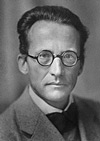 E. Schrodinger
Nobel Prize laureate 1933
E. Schrodinger
Nobel Prize laureate 1933 A. Einstein Nobel Prize laureate 1921
 Last change: 5 February 2001