 The Born-Oppenheimer approximation
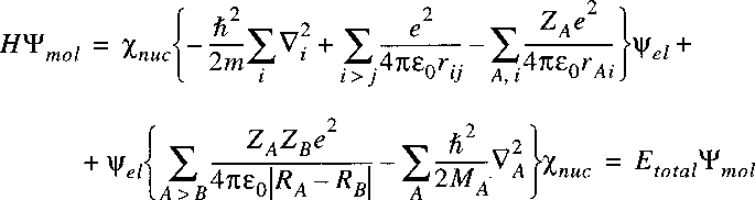
The Hamiltonian for a system of nuclei and electrons can be written as:
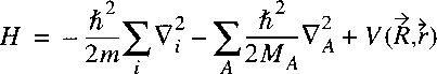
where the summation i refers to the electrons and A to the nuclei.
The first term on the right corresponds to the kinetic energy of the electrons,
the second term to the kinetic energy of the nuclei and the third term to the Coulomb energy,
due to the electrostatic attraction and repulsion between the electrons and nuclei.
The potential energy term is equal to:
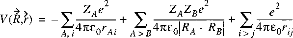
The negative terms represent attraction, while the positive terms represent Coulomb-repulsion.
Note that a treatment with this Hamiltonian gives a non-relativistic description of the molecule,
in which all spin-effects have been ignored.
Now assume that the wave function of the entire molecular system is separable and can be written as:
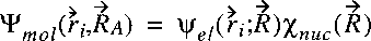
where Psiel represents the electronic wave function and
Chinuc the wave function of the nuclear motion.
In this description it is assumed that the electronic wave function can be calculated
for a particular nuclear distance R. Then:
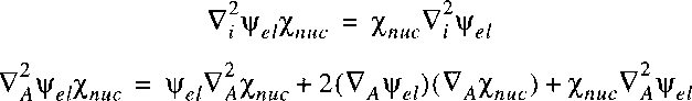
The Born-Oppenheimer approximation now entails that the derivative of
the electronic wave function with respect to the nuclear coordinates is small,
so is negligibly small.
In other words this means that the nuclei can be considered stationary,
and the electrons adapt their positions instantaneously to the potential field of the nuclei.
The justification for this originates in the fact that the mass of the electrons is several
thousand times smaller than the mass of the nuclei.
Indeed the BO-approximation is the least appropriate for the light H2-molecule.
If we insert the separable wave function in the wave equation:

then it follows:
The wave equation for the electronic part can be written separately and solved:
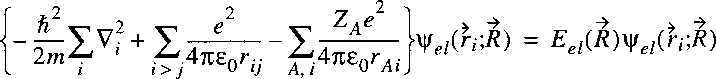
for each value of R.
The resulting electronic energy can then be inserted in the wave equation
describing the nuclear motion:

We have now in a certain sense two separate problems related to two wave equations.
The first relates to the electronic part, where the goal is to find the electronic wave function
and an energy.
This energy is related to the electronic structure of the molecule analogously to that of atoms.
Note that here we deal with an (infinite) series of energy levels, a ground state and excited states,
dependent on the configurations of all electrons.
By searching the eigen values of the electronic wave equation for each value of R we find a
function for the electronic energy, rather than a single value.
Solution of the nuclear part then gives the eigen functions and eigen energies:

In the BO-approximation the nuclei are treated as being infinitely heavy.
As a consequence the possible isotopic species (HCl and DCl) have the same potential in the BO-picture.
Also all couplings between electronic and rotational motion are neglected.
Potential energy curves
The electrostatic repulsion between the positively charged nuclei:
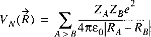
is a function of the internuclear distance(s) just as the electronic energy.
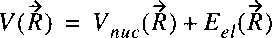
These two terms can be taken together in a single function representing the
potential energy of the nuclear motion:
In the case of a diatom the vector-character can be removed;
there is only a single internuclear distance between two atomic nuclei.
In the figure
potential energy curves
are displayed, for ground and excited states.
Note that:
 at small internuclear separation the energy is always large,
due to the dominant role of the nuclear repulsion
at small internuclear separation the energy is always large,
due to the dominant role of the nuclear repulsion
it is not always so that the electronic ground state corresponds to a bound state
electronically excited states can be bound.
Electronic transitions can take place, just as in the atom, if the electronic configuration
in the molecule changes.
In that case there is a transition from one potential energy curve in the molecule to
another potential energy curve. Such a transition is accompanied by absorption or
emission of radiation; it does not make a difference whether or not the state is bound.
The binding (chemical binding) refers to the motion of the nuclei.
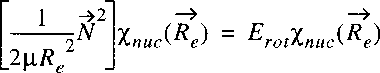
Rotational motion in a diatomic molecule
Starting point is the wave equation for the nuclear motion
in the Born-Oppenheimer approximation:
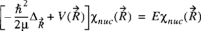
where, just as in the case of the hydrogen atom the problem is transferred to one of a reduced mass.
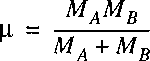
Note that mu represents now the reduced mass of the nuclear motion:
Before searching for solutions it is interesting to consider the similarity between
this wave equation and that of the hydrogen atom.
If a 1/R potential is inserted then the solutions (eigenvalues and eigenfunctions)
of the hydrogen atom would follow. Only the wave function has a different meaning:
it represents the motion of the nuclei in a diatomic molecule.
In general we do not know the precise form of the potential function V(R) and also
it is not infinitely deep as in the hydrogen atom.
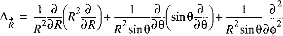
Analogously to the treatment of the hydrogen atom we can proceed by writing the
Laplacian in spherical coordinates:
Now a vector-operator N can be defined with the properties of an angular momentum:
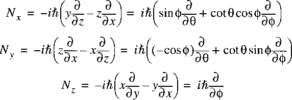
The Laplacian can then be written as:
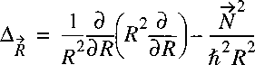
The Hamiltonian can then be reduced to:
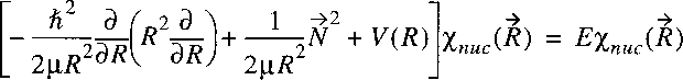
Because this potential is only a function of internuclear separation R,
the only operator with angular dependence is the angular momentum N2,
analogously to L2 in the hydrogen atom.
The angular dependent part can again be separated and we know the solutions:
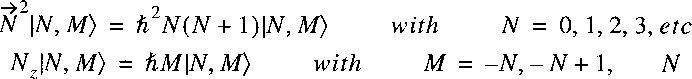
The eigenfunctions for the separated angular part are thus represented by the
well-known spherical harmonics:

and the wave function for the molecular Hamiltonian:
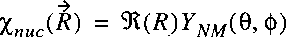
Inserting this function gives us an equation for the radial part:
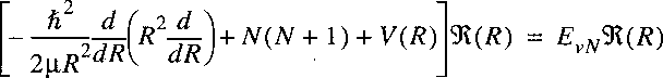
Now the wave equation has no partial derivatives, only one variable R is left.
The rigid rotor
Now assume that the molecule consists of two atoms rigidly connected to each other.
That means that the internuclear separation remains constant, e.g. at a value Re.
Since the zero point of a potential energy can be arbitrarily chosen
we choose V(Re)=0.
The wave equation reduces to:
The eigenvalues follow immediately:
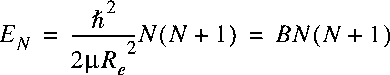
where B is defined as the rotational constant.
B is closely related to the
moment of inertia of the molecule.
Hence a ladder of
rotational energy levels appears in a diatom.
Note that the separation between the levels is not constant,
but increases with the rotational quantum number N.
For an HCl molecule the internuclear separation is Re=0.129 nm;
in fact this
bond length is derived from the rotational spacings as observed in
pure rotational spectra.
Deduce that the rotational constants 10.34 cm-1.
This analysis gives also the isotopic scaling for the rotational levels of an isotope:

 Advanced topic:
The elastic rotor; centrifugal distortion
Advanced topic:
The elastic rotor; centrifugal distortion
Vibrational motion in a non-rotating diatomic molecule
If we set the angular momentum N equal to 0 in the Schrodinger equation for the radial part and
introduce a function Q(R) with R(R)=Q(R)/R
than a somewhat simpler expression results:
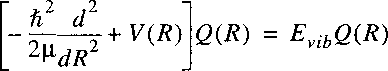
This equation cannot be solved straightforwardly because the exact shape of the
potential V(R) is not known.
For bound states of a molecule the potential function can be approximated with a quadratic function.
Particularly near the bottom of the potential well that approximation is valid (see figure).
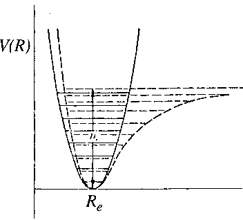
Near the minimum R=Re a Taylor-expansion can be made, where we use
r = R - Re:
and:
Here again the zero for the potential energy can be chosen at Re.
The first derivative is 0 at the minimum and k is the spring constant of the vibrational motion.
The wave equation reduces to the known problem of the
1-dimensional quantum mechanical harmonic oscillator:
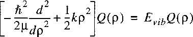
The solutions for the eigenfunctions are known:

where Hv are the Hermite polynomials; the energy eigenvalues are:
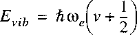
with the quantum number v that runs over values v=0,1,2,3.
From this we learn that the vibrational levels in a molecule are equidistant and that there is
a contribution form a zero point vibration.
The averaged internuclear distance can be calculated for each vibrational quantum state from the
expectation values using the known
wave functions.
Note that at high vibrational quantum numbers the largest density in the
probability distribution
is at the classical turning points of the oscillator.
Note also that there is a zero-point energy of the lowest vibrational level
above the minimum of the potential well, which may be related to the
uncertainty principle.
The isotopic scaling for the vibrational constant is:

Note also that the zero point vibrational energy is different for the isotopes.
The
Bond force constant can be derived from vibrational spectra,
as in the case of
HCl or
HBr.
Advanced topic:
Anharmonicity in the vibrational motion
In the figure below the potential and the vibrational levels for the
H2-molecule are shown.
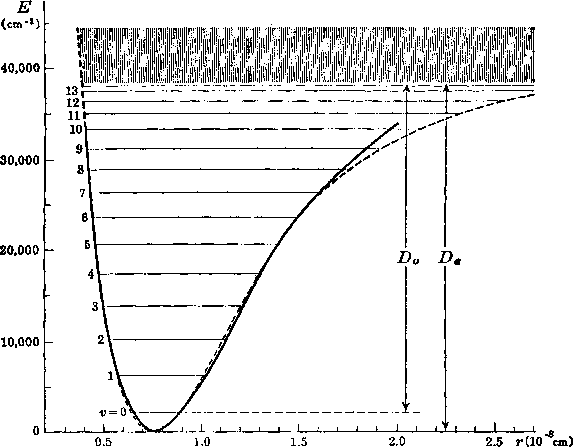
H2 has 14 bound vibrational levels.
The shaded area above the dissociation limit contains a continuum of states.
The molecule can occupy this continuum state!
For D2 there are 17 bound vibrational states.
A potential energy function that often resembles the shape of bound electronic state
potentials is the
Morse Potential defined as:
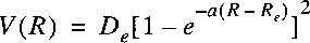
where the three parameters can be adjusted to the true potential for a certain molecule.
One can verify that this potential is not so good when approaching infinity.
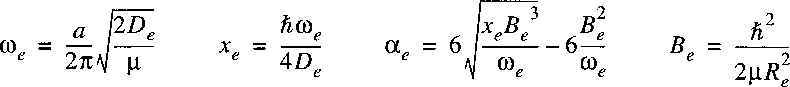
By solving the Schrödinger equation with this potential one can derive the spectroscopic constants:
A procedure that is often used for representing the rovibrational energy levels within a
certain electronic state of a molecule is that of Dunham, first proposed in 1932:
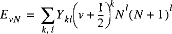
In this procedure the parameters
Ykl are fit to the experimentally determined energy levels;
the parameters are to be considered a mathematical representation,
rather than constants with a physical meaning.
Nevertheless a relation can be established between the
Ykl
and the molecular parameters Be, De, etc.
In approximation it holds:

Energy levels in a diatomic molecule: electronic, vibrational and rotational
In a molecule there are electronic energy levels, just as in an atom,
determined by the configuration of orbitals.
Superimposed on that electronic structure there exists a structure of
vibrational and rotational levels.
Transitions between levels can occur, e.g. via electric dipole transitions,
accompanied by absorption or emission of photons.
Just as in the case of atoms there exist selection rules that
determine which transitions are allowed.
 Last change: 27 February 2001
at small internuclear separation the energy is always large,
due to the dominant role of the nuclear repulsion
it is not always so that the electronic ground state corresponds to a bound state
electronically excited states can be bound.
Advanced topic:
The elastic rotor; centrifugal distortion
Advanced topic:
Anharmonicity in the vibrational motion
A potential energy function that often resembles the shape of bound electronic state
potentials is the
Morse Potential defined as:
where the three parameters can be adjusted to the true potential for a certain molecule. One can verify that this potential is not so good when approaching infinity. By solving the Schrödinger equation with this potential one can derive the spectroscopic constants:
A procedure that is often used for representing the rovibrational energy levels within a
certain electronic state of a molecule is that of Dunham, first proposed in 1932:
In this procedure the parameters Ykl are fit to the experimentally determined energy levels; the parameters are to be considered a mathematical representation, rather than constants with a physical meaning. Nevertheless a relation can be established between the Ykl and the molecular parameters Be, De, etc. In approximation it holds: