Laser Doppler Anemomentry
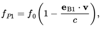
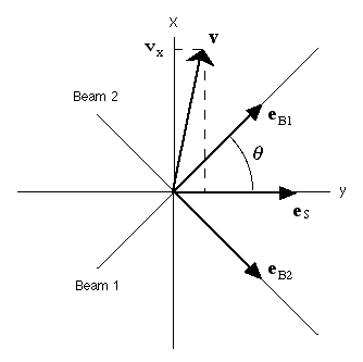
The theoretical background of LDA can be based on either relativistic or classical arguments. From a relativistic point of view one uses the frequency shift that light waves undergo when scattered by moving particles, i.e. the Doppler shift. Assume a particle is moving along with the flow in a fluid with velocity v (see fig. 1.1). If the particle crosses a beam 1 of monochromatic light with frequency f0, it receives the light at a shifted frequency given by:
Liquid Flow through a Pipe
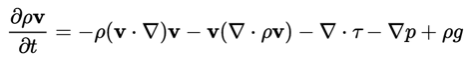
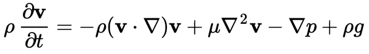
The characteristics of flows are studied in the field of fluid dynamics. The most general description of a flow is known as the Navier-Stokes equation:
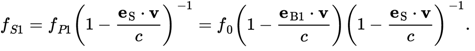
where c is the speed of light and eB1 is a unit vector in the direction of the light beam. The light emitted by a moving particle or the scattered light received by an observer at rest will undergo an additional frequency shift given by:
This equation relates the particle velocity v to a measurable shifted frequency fS1. It does not however allow to distinguish between particles crossing the beam at different locations, so the spatial resolution will be poor.
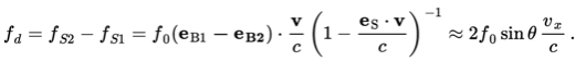
If one takes the first beam to be coherent and monochromatic and combines this beam with a second equivalent beam, this drawback can be eliminated. To this end one creates an intersection of the two beams. The scattered light originating from this intersection, also called the measurement volume, will form a linear combination of the scattered light resulting from beam 1 and that of beam 2. As the directions of the two beams differ, so will the frequencies fS1 and fS2. The addition of waves of equal intensity and differing frequency yields a light wave with an amplitude modulated with frequency (fS2 - fS1) / 2 and an irradiance modulated with a frequency (fS2 - fS1). The latter is generally called the beat frequency, but in the context of LDA it is also called the Doppler frequency. One finds that this Doppler frequency fd of the scattered light is given by:
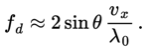
Here it is assumed that , which in approximation is correct. In terms of wavelength eq. (1.3) may be rewritten as:
This establishes the linear relationship between the Doppler frequency fd and component vx of the particle velocity in the direction perpendicular to optical axes of the lenses of the system, from here on called the optical axis of the system.
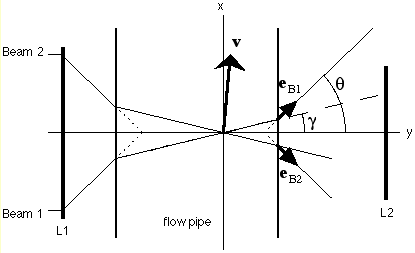
Figure 1.1: The geometry of the LDA measurement. Each of the beams is incident under an angle with the 'optical axis' of the system, along the y-axis. The intensity of the light scattered in this direction by some particle with velocity v is modulated with a the Doppler frequency that is proportional to the inner product of the particle velocity and the vector (eB1 - eB2). Note that this implies that the Doppler frequency is it is proportional to the x-component of the particle velocity.
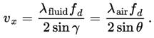
It may be noted that the relation presented in eq. (1.4) only relates the Doppler frequency to the absolute value of the velocity of flow in the x-direction. The system therefore can not measure any difference between velocities in positive and negative x-direction. Generally the direction of flow is known, but one may be confronted with a situation where it is necessary to distinguish the direction of flow. This can be achieved by the application of two beams of differing frequency. Suppose that the frequency of beam 1 is given by and that the frequency of beam 2 is given by . This implies that eq. (1.1) is to be rewritten and following the argument above this yields a Doppler frequency given by:
If the velocity of the particle is zero, the Doppler frequency will be equal to the difference between the frequencies of beam 1 and beam 2. For the system to be sensitive to negative velocities as well, one should choose such that fd will still be positive for the smallest velocities.
From a classical point of view the two beams will interfere at the intersection or within the measurement volume. This results in a series of light and dark surfaces or fringes, parallel to the optical axis of the system. A particle passing these fringes will scatter light with a frequency equal to that of the illumination, i.e.:
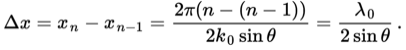
where is the spatial period of the intensity in the direction perpendicular to the optical axis of the system. This spatial period is the spatial period of the intensity of the combined beams, i.e. of the beat signal. Since the spatial pattern is independent of time this yields:
Here is the wavenumber [m-1] of the respective beams and .The spatial period of this cosine-term then is given by:
Combining eq. (1.6) and (1.8) this finally yields the same result as eq. (1.4).
Finally some considerations on the geometry of the LDA system with respect to the measurement volume are worth mentioning. For the determination of the position of the measurement volume in the flow pipe the propagation of the incident laser beams is to be corrected for the refraction of the beams. In fig. 1.2 the situation is sketched for a horizontally positioned flow pipe with incoming laser beams in the plane of the sketch. With Snell's law one may therefore rewrite eq. (1.3) as:
Furthermore one may extend the trajectory of the beams at either side of the flow pipe as if there were no flow pipe. The two intersections then form the virtual measurement volumes for an observer at the position of lenses L1 and L2 respectively. These two positions are fixed with respect to the lenses, irrespective of the location of the flow pipe. This will turn out to come in handy in the design of the system.
Figure 1.2: The path of two laser beams through a flow pipe. The actual geometry of the measurement volume is based on angle , which on its turn is related to the angle through Snell's law as in eq. (1.9).
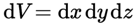
This equation may basically be considered as a balance of forces over a cubic volume element . In this respect the Navier-Stokes equation can be interpreted as a formulation of the second law of Newton, with on the left hand side the change of momentum in the volume dV due to the forces exerted on this volume that are summed on the right hand side. The first two terms on the right quantify the inertia forces. The third term stands for the viscous forces that may be interpreted as the frictional forces acting on the volume. The forth and the fifth term represent the pressure forces and the gravity force respectively.
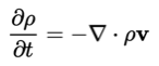
In a first approximation the Navier-Stokes equation can be simplified through the specification of the fluid that is dealt with. Assuming incompressibility, one may take the mass balance into consideration:
Furthermore if the equation is applied to a Newtonian fluid, the viscous forces are linearly related to the spatial derivative of the velocity through the dynamic viscosity. For other classes of fluids different and generally more complicated relationships between viscous forces and the spatial derivative of the velocity have been established. For the case at hand however the resulting equation is:
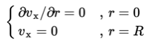
Integrating eq. (1.4) with boundary conditions
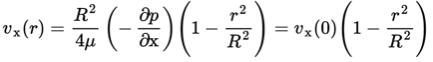
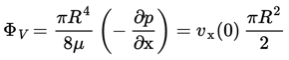
This flow pattern is also known as Poiseuille flow and shows that the velocity distribution for a laminar flow in a horizontal cylindrical pipe is parabolic. The volumetric throughput then is found through integration over the cross section of the flow pipe (Hagen-Poiseuille law):
Here is the dynamic viscosity of the fluid. For relatively slow moving fluids one may assume a laminar, or layered, flow pattern. In this model it is assumed that the flow pattern consists of a number of layers parallel to the velocity, that differ in velocity. The velocity is assumed to be zero at the wall and increases with distance from this wall. Assuming a stationary laminar flow in a cylindrical pipe, eq. (1.12) can be solved analytically.
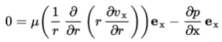
A stationary flow is assumed so that the time dependence on the left hand side of the equation is zero. Furthermore the acceleration g is a vector perpendicular to the direction of flow so that gravity can not lead to accelerations in the direction of flow. The measurements will however only be performed at the height of the axis of the pipe so that the last term can be left out of the equation as well.
Finally the gradient operator and the Laplace operator for cylindrical coordinates can be applied, where the angular dependence can be left out for reasons of axial symmetry. Since the velocity is independent of the axial variable x, its derivative with respect to x is zero. The same goes for the pressure with respect to the radius. Furthermore the velocity component v, in the direction of the radius is zero so that the final result is:
The former derivation is applicable as long as the laminar model can be assumed. For higher velocities however a new regime is entered, known as turbulence. Characteristic for turbulence is that viscous forces are small compared to the inertia forces. The inertia forces may in this context be taken to be a measure of the kinetic energy contained in a flow. The viscous forces on the other hand, are responsible for the distribution of the kinetic energy in the flow. For a laminar flow the kinetic energy is passed from layer to layer through the viscous forces. If the viscous forces are too small compared to the kinetic energy present, another mechanism arises. A spatially and temporally unstable pattern of eddies arises where large eddies transfer their kinetic energy to smaller ones and these again to even smaller ones. This yields an ever changing flow pattern that spreads the kinetic energy in a very effective manner. The direction and magnitude of the velocity vector then are no longer unambiguous and therefore eq. (1.12) can no longer be solved analytically.
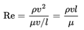
To describe the regime of the flow use is made of the Reynolds number Re defined as the dimensionless ratio of the inertia forces and the viscous forces;
where l is some length characteristic for the dimensions of the flow, which in this case is the diameter of the flow pipe.
Roughly speaking, for a straight cylindrical flow pipe the flow is laminar for Re < 2000. If 2000 < Re < 2500 the regime may change to the turbulent. A range is given because other phenomena then the viscous and inertia forces may be of influence. Here one may think for instance of oscillations introduced by the pump since influences like these promote the instability of the laminar flow.