Experimental design and measurement

2. Experimental design and
measurement

System Design

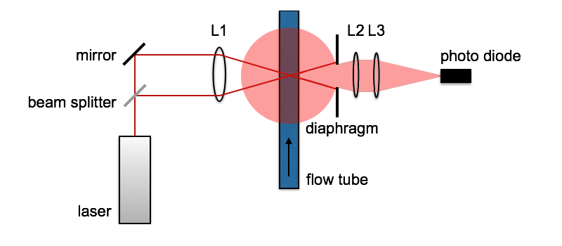
Many varieties of LDA systems are possible. A common and general set up, as used in the physics lab at the VU (see fig. 2.1), will be discussed here . This LDA system is a single frequency, single component LDA system with forward-scattered detection. In other words the system allows for the measurement of the absolute value of one velocity component at a time, by measurement of the forward scattering. Some remarks on other options will be made in the following discussion as well.
In the most general sense the system is composed of three main parts. The first consists of the illuminating component that is used to create a measurement volume. The second part of the system consist of the optical detection apparatus with the objective of measuring the scattered light and the last part is the signal processing component that is used for the processing of the output of the photo diode.

Optimization

Optimization of the illuminating system comes down to optimization of the amplitude, volume and the regularity of the fringe pattern. Various points of interest for signal optimization have been discussed in the section on system design already:

For an optimal signal-to-noise-ratio the intensity of the two beams should differ less than some 5 %.
For a small measurement volume the angle should not be too small, but preferable such that the two beams fall within the paraxial region.
For a regular fringe pattern, i.e. for the fringe gradient to approach zero, the beams should fall within the paraxial region of the first lens resulting in a relatively small angle.
One may check the quality of the measurement volume in terms of fringe gradient by performing a measurement with use of a rotating wire, as discussed in the section on complications.

Apart from these constraints, the alignment of the two beams should be optimized. This may for instance be done through moving a screen over a distance over the optical bench. The point of illumination should remain in place.

Optimization of the optical detection system comes down to maximizing the amount of scattered light that falls into the photodiode. Some conditions for optimization of the optical detection system have been discussed in the section on system design already. It was mentioned there that for ease of alignment it is useful to configure the two lenses in such a way that the focal length of the second lens equals the distance between the second virtual measurement volume and the second lens. Furthermore the focal length of the third lens should equal the distance between the photodiode and the third lens.

For the optimization of the signal processing, a good signal-to-noise-ratio should be pursued. It is mainly a matter of getting a good signal-to-noise-ratio through adjustment of the diaphragm, the offset of the amplifier and the amplification. What this signal looks like is discussed in the section on signal processing and data analysis.

Procedure

The procedure to perform a measurement consists of the subsequent steps:

Optimize the general parameters of the instrument as described above
Make an estimate of all the relevant variables and their inaccuracies
Perform a series of spectral measurements for various flow velocities
Estimate the center frequencies and the standard deviation of each of the spectral peaks
Calculate the relevant variables from these data
Perform an error analysis
Graph or tabulate the relevant data and their respective uncertainties
Draw conclusions

Figure 2.1: Schematic of the experimental setup. The overlapping laser beams form the measurement volume. Light waves impinging on small particles are scattered through Mie scattering. The diaphragm blocks the laser beams. Scattered light passing through the diaphragm is focussed on a photo diode.

Illumination

As discussed in the theory a coherent and monochromatic beam is required so that here a 5 mW He-Ne laser is used. The beam is split with a beam splitter. The resulting two beams should be equivalent or nearly equivalent in intensity. This yields the highest degree of contrast between the fringes in the measurement volume and thus the highest amplitude for the signal so that the signal-to-noise ratio is maximized. If the amplitudes of the two beams differ less than some 5% the contrast is virtually maximal. An optical density filter may be used to correct for any larger differences.
The two beams should be aligned in parallel, so that a lens L1 can be used to let the beams intersect. The beams are to pass the lens equidistantly from the optical axis of the lens so that the angle is equal for the two beams (see fig. 2.1). This angle is determined by the distance between the beams and the focal length of lens L1.
An appropriate choice for this angle is not unambiguous. In the first place the choice for some angle will have consequences for the intensity of the signal. Since the intensity for forward scattering is generally high enough for a good signal-to-noise ratio, these considerations will not be discussed here. The choice for a specific angle however also has consequences for the size and formation of the measurement volume.
In the first place a smaller angle results in a larger size of the measurement volume in the direction of the optical axis. Since the velocity gradient in this direction is non-zero this will result in a certain distribution in the velocities measured and thus in a broadening of the Doppler frequency. A smaller angle may therefore yield a larger uncertainty in the Doppler frequency, so a large angle may be preferable. A large angle on the other hand implies that the two beams may no longer fall within the paraxial region and therefore spherical aberation may occur (see Complications).

Optical Detection

The aim of the optical detection system is to measure the scattered light waves originating from the measurement volume. The light waves that impinge on the particles are scattered through Mie scattering. This type of scattering occurs when the size of the scattering particles is comparable to or larger than the wavelength of the illuminating light waves. The detection system can be set up to measure the scattered light in any direction. Generally the intensity of the scattered light is the highest in the forward direction, so that often forward scattering is detected. If backward scattering is measured however, high power lasers are needed since the intensity in this direction is generally low. The advantage of such a set up is that the illuminating system and the detection system can be integrated.

For forward-scattered detection as in fig. 2.1 a simple arrangement of two converging lenses may be used to increase the light gathering power of the system. The signal is detected using a photo diode. A diaphragm may be positioned between the measurement volume and the second lens so that mainly the scattered light originating from the measurement volume enters the system. One may choose for a set up as suggested in fig. 2.1 Here the second virtual measurement volume is located at the focal point of lens L2. This yields an image located at infinity that on its turn is projected on the focal plane of lens L3. This configuration has the advantage that it is relatively easy to align.

Signal Processing

The output signal of the photo diode may be processed using an amplifier, an A/D-converter and a digital processor. It is useful to apply an amplifier that allows for correction of bias in the signal since the intensity of the scattered light may vary notably for different circumstances. Furthermore the digital processor should have a high sampling rate and an option to perform Fourier transforms so that spectral measurements can be made.

Flow Circuit

In general the object of measurement of the LDA system is some flow. In a first approach however it is useful to measure a controlled flow. This offers the opportunity to calibrate the system.
To this end a relatively simple option is to apply the LDA measurements to water, or any other fluid, in some flow circuit. A glass pipe may offer a measurement window and if a valve and flowmeter are implemented in addition to a stable pump, most relevant parameters are controlled. In addition it may also be useful to have a cooling circuit (a simple cooling circuit connected to a running tap will do) and a thermometer at one's disposal, since the dynamic viscosity mu can be highly temperature dependent.
The fluid should contain particles that have sizes comparable to the spatial period of the fringe pattern as given by eq. (1.8). In plain tap water particles with sizes in the order of mm are present. When using a fluid that does not contain such particles seeding may be needed. In that case one may add some flower, milk or Detol.

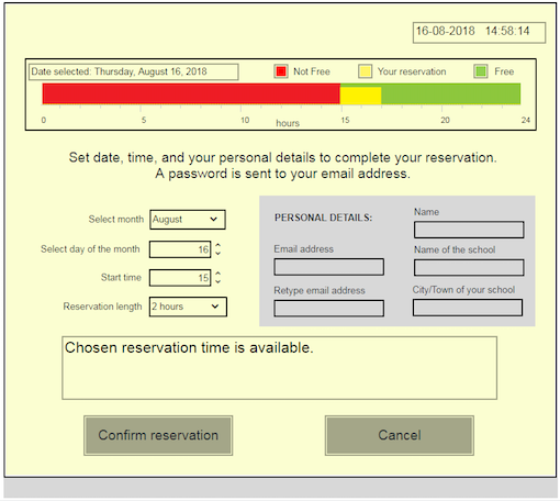
At the left bottom of the window select a month and day to schedule your experiment. A reservation always lasts for 1 or 2 hours. You can log in for the start of the hour that you reserve. The bar at the center of the screen shows available time slots for the day you selected. The experiment can be reserved 24 hours a day.

Please fill out the remaining parts. Make sure to enter a valid e-mail address. After completing the data you will receive an e-mail at the given address with the timeslot and password to conduct the experiment.

Start the experiment

On the scheduled day and time log in to conduct the experiment through http://pc-008368.clients.vu.nl/lda/lda.html.
The crossing laser beams used in the LDA experiment can be viewed at http://pc-021444.clients.vu.nl/.
Click on LOGIN for experiment, which results in the screen shown in figure 2.4.

Making a reservation for the Laser Doppler Anemometry experiment

The remote lab can be reached at: http://pc-008368.clients.vu.nl/lda/lda.html

You will obtain the screen shown in figure 2.2 (if not, or in case you get the message that the experiment is offline, please send an e-mail to Jan Mulder (j.m.mulder@vu.nl).

Figure 2.2: Screen for reservation of the remote lab

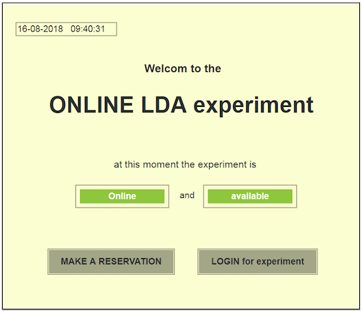
Before you login to conduct the experiment you first need to make a reservation. This is to ensure that only one user can run the experiment at the time. Click on MAKE A RESERVATION to plan your reservation. The screen in figure 2.3 will be shown:

Figure 2.3: Screen for time reservation

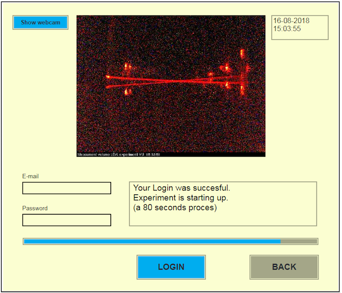
Figure 2.4: Login screen to start remote lab

Enter your e-mail address and password. The system will start up. If you click on Show Webcam you can view the crossing laser beams, which are used for the LDA experiment. After start up the control panel shown below in figure 2.5 will appear:

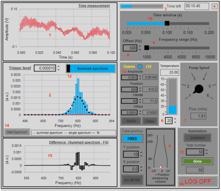
Figure 2.5: The LDA web interface. For details see text.

This graph shows the signal recorded with the AC photo diode.
This graph shows the frequency spectrum (Fourier transform, FT) of the time spectrum (1). Depending on the setting of (12) a single spectrum or a summed spectrum is shown.
The timer shows how much longer you can continue. From the moment your reservation starts you get 55 (or 115) minutes to conduct the experiment.
A light signal will be given when only 5 minutes are left. This means you need to wrap up your experiment.
Here you can set the location of your measuring volume within the tube. The Xpos and Ypos settings will only be adjusted when you press Do MOVE. During movement of the tube the FIXED indicator alternatively lights up in red and blue. Note: moving the tube takes time. When the indicator FIXED stays blue the tube reached its location.
Here you can set the temperature of the water running through the tube. Cooling and heating of water takes time. The indicator on top shows the actual temperature of the water. The highest temperature you can set is 50 degrees Celcius.
Here you can adjust the flow rate of the water by turning the knob. The indicator shows the actual flow rate in mL/s.
The FT shown in (2) will show a strong signal near 0 Hz, which due to autoscaling of the graph can make it difficult to see the actual signal. Using an offset you can hide the peaks at the start. So this setting determines the start value of your graph.
This setting determines the upper range for the FT spectrum (2).
This determines the time windows used for the FT. When you increase the value narrower peaks will be shown in the FT at the expense of longer measurement times.
You can sum the FT spectra. The indicator below shows how many spectra have been summed. When the number set has been reached the DONE indicator lights up. This may take some time. You can (re)start the summing at any convenient time. The trigger level (in the FT panel (2)) determines whether of not a single frequency measurement is shown and summed. The trigger level can be used to suppress noise. A too high value can prevent measurements to be included though (when single spectrum is chosen the FFT will remain empty when the trigger level is set too high).
You can either display a single frequency spectrum or the summed spectrum using the slider switch.
The summed frequency spectrum can be fitted with a Gaussian profile. In order to do so you need to set initial values. The cursor in the frequency spectrum window can be used to find appropriate initial settings. Press DoFit to start the fitting. The fit result will be added to the graph as a black dotted trace.
The measurement data collected will be send to you by e-mail when you click this button. This is only required if you want to use a separate data analysis software.
When you perfom a Gaussian fit the graph shown here will show the residue of the fit.
Click here to log off to end the experiment.

IT IS RECOMMENDED TO MAKE SCREEN SHOTS OF THE LDA WEB INTERFACE WITH THE FIT RESULTS
UNLESS YOU EXPORT YOUR DATA AND PERFORM AN ANALYSIS USING YOUR OWN DATA ANALYSIS SOFTWARE