In principle the error analysis allows for the estimation of uncertainties in the measurements due to uncertainties of the relevant parameters. Here the relevant parameters follow from the theory described. In the derivation of the equations however some assumptions have been made that can lead to complications that do not follow from the error analysis.
One problem that may occur originates in the assumption that the particles have the same velocity as the fluid. For gases one may think of the Maxwell distribution of speeds that causes problems, since these velocities may be comparable to the convective flow under study. These velocities are of random direction so they may yield a heavy broadening of the spectral peak around the Doppler frequency. With respect to the velocity measurements of convective flows in liquids one may think of Brownian movement, but the order of the velocities that arise due to this phenomenon is generally much lower than that of of the convective flow. It is questionable however whether the particles will follow the flow with the same velocity as the liquid. Their behaviour in this context may very well depend on their masses and volumes. If this is the case a distribution in the particle sizes in the fluid will reflect upon the distribution of spectral intensity around the Doppler frequency.
Another assumption that may lead to inaccuracies is that the measurement volume is taken to be a singularity. In reality the measurement volume is a small volume and the velocity of flow within this volume may differ from one point to the other. In otherwords if the gradient of the velocity is large enough there may be a significant spread in the velocities and thus a resulting spread in the Doppler frequency. whether the gradient is large enough depends on the width of the measurement volume in the direction of the gradient, i.e. in the radial direction. In principle the volume of the measurement volume can be very small due to focusing of the beams. According to first order optical theory all rays parallel to the optical axis, incident on a converging lens should pass through the focal point of the lens. This is also true for the margins of a single laser beam. In other words first order optical theory theory suggests that the width of the beams at the focal point approaches zero and the measurement volume is a singulary. In reality the phenomenon of spherical aberration results in a finite measurement volume.
Figure 5.1 : The focusing of a beam, subject to spherical aberration
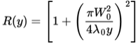
Only when the cross section of the surface of a lens describes a cartesian oval, then the focal point will be one and the same for any incident ray. Since the fabrication of such lenses is expensive, most optical lenses have spherical surfaces. For rays passing a lens close to the optical axis the spherical surface does not deviate too much from a cartesian oval, but the more off-axis the point of incidence the more severe the deviation. For a converging lens the result is that the focal point depends on the point of incidence, such that the focal length decreases with increasing distance between the point of incidence and the optical axis. This phenomenon is known as spherical aberration. In figure 5.1 a schetch of a wide beam centered at the optical axis and subject to spherical aberration is shown. Since there is not a single focal point, a certain minimum width of the converging beam is located at the position of the focal plane of the marginal rays. This is called the waist of the beam and is described by:
Here f is the focal length of the lens L1. In fig. 5.2 the sketch represents the LDA configuration with two off-axis beams incident on the lens. The measurement volume is indicated in red. Clearly the waist of the beam in figure 5.1 and eq. (5.1) is an upper limit for the width of the measurement volume in the direction of the flow. The problem is however the width in the direction of the optical axis, since the velocity gradient is non-zero in this direction. The width of the measurement volume in the y -direction is equal to the distance between the focal points of the margins of the laser beams.
Figure 5.2 : The width of the measurement volume due to spherical aberration
Another result of the spherical aberration may be quite influential. The wavefronts of the laser beams after lens L1 show some bending with a radius given by:
Here R approaches infinity for y approaching zero so that the wavefronts approach planar wavefronts. Here y has its origin in the focal point, so that at that point the waves become planar. If spherical aberration leads to off-axis focussing, the wavefronts will show some bending in the measurement volume. The result may be a severe distortion of the fringe pattern, as sketched in figure 5.3. In the left sketch, planar wave fronts are asumed, and a nice and regular fringe pattern is the result. In the right sketch spherical wavefronts are assumed, with decreasing radius in the direction of propagation, as follows from eq. (5.2). This turns out to yield a fringe pattern that has a tendency to 'fan out'. Furthermore the fringes are subject to bending as well. The result therefore is a (non-linear) gradient in the fringe pattern yielding a broadening in the Doppler frequencies measured.
One could try to calibrate the system through measurement of this fringe gradient. To measure the fringe bias qualitatively one may use a wire on a rotating disc, simulating a particle of known size and velocity. This results in a nice pedestal wave with the signal with the Doppler frequency superposed on it. By passing the wire on different positions through the measurement volume one may be able to measure different Doppler frequencies for various positions. If detected however little more than improvement of the quality of lens L1 can be done. Theoretically one could improve the alignment of the system, but the alignment takes place on the mm-scale, whereas the scale of the fringe gradient is comparible to that of thewavelenght of the laser, i.e. in nm.
Figure 5.3 : Sketch of the measurement volume without fringe gradient (left) and with a fringe gradient (right).
A third problem that may arise is sampling bias. Sampling bias occurs when any of the relevant electronic equipement is unable to keep up with the Doppler frequency. If the sampling rate is too low, the measurement could lead to any result but not a useful one. In general the Doppler frequencies will be low enough, but for the special case of high velocities one should realize that sampling bias may occur. The same holds for measurements performed with beams of differing frequencies, as suggested in eq. (1.5). Since photo diodes generally are insensitive to frequencies higher then some 50 kHz this shows one of the limitiations of the LDA method.