Introduction
The signal is composed of low frequency background noise, the Doppler frequency and high frequency components in the order of the frequency of the laser beam.
The low frequency noise can be the result of some other light source, the vibrations of the pump, or purely electronic noise. Generally it increases with decreasing frequency and it is particularly high for frequencies below the 2 kHz.
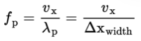
The Doppler signal has been discussed briefly in the theory. The addition of waves of equal intensity and differing frequency yields a light wave with an irradiance that is modulated with the so-called beat frequency. There is however not continuously a scattering particle present. The Doppler signal increases in intensity when a particle enters the measurement volume up to the center and decreases again upon leaving the measurement volume. This is the result of the Gaussian distribution of the intensity of the laser beams, that reflects on the intensity distribution of the measurement volume. For a single particle this results in an additional modulation with a 'frequency' that corresponds to:
Software
The data analysis software to perform a Gaussian fit on the summed frequency spectrum, is included in the Remote Lab software and can be performed during the experiment. The experiment data can also be processed after the experiment when you opt to e-mail the experimental data to yourself in a data analysis program of your own choice.
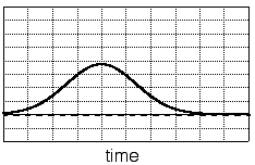
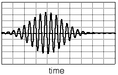
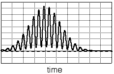
(a) Pedestal wave (b) Doppler wave (c) Signal burst
Figure 3.1: Sketches of the components of the measured signal as shown in fig. 3.2. The pedestal wave (a) results from the intensity increase and decrease of the scattered light when a particle crosses the measurement volume.
The Doppler signal (b) results from the interference of the scattered light originating from the two beams.
Finally the signal burst (c) is the resulting signal, i.e. the Doppler wave superposed on the pedestal wave.
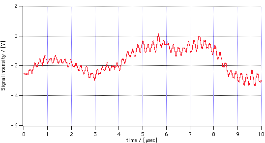
Figure 3.2 : An example of an actual measured signal. The higher frequency component corresponds to the Doppler frequency, whereas the low frequency component is in the order of the Pedestal wave.
After a clearly established measurement of the signal burst on a regular basis one can start the spectral measurements. These are to be averaged over a temporal period that is substantially larger than the period of the occurence of a signal burst, since it is highly dependent of the velocity of passing particles (see complications) and the regularity of the fringe pattern (see complications).
Once a series of spectra is obtained, one may estimate the center frequency and the width of the spectral peaks. The next step is an error analysis, including the propagation errors that result from the calculation of velocity. This should include all relevant parameters like the distance between the beams passing lens L1, the focal length of lens L1, the position of the measurement volume etc.
Here the 'wavelength' is equal to the width of the measurement volume in the direction of the flow. The Doppler signal itself is always accompanied by this 'carrier wave' , also called the pedestal wave. The result is a so-called signal burst that is composed of the pedestal wave, with the Doppler wave superposed on it. A scetch of these signals is presented in fig. 3.1. The signal burst manifests itself as a highly recognizable burst, both for its frequency as for its intensity. This is a very useful property when one is adjusting the data processing instrumentarium through adjustment of the diaphragm, the bias of the amplifier and the amplification and it is therefore advisable to perform the optimazition of these while keeping an eye on the signal in the time domain. This should be done for each measurement performed, since the intensity of the signal may vary heavily for changing circumstances. This implies that the signal intensity may be so low that nothing is detected or that the photodiode may suffer from an overload. In the first case there will hardly by any signal in the frequency dimension, but in the second case there will be additional frequency components present. The occasional overload may be interpreted as an additional square wave. Since this type of waves is built up of a series of high frequency components the square wave will, under a Fourier transform, result in this decomposition.
Apart from the low frequency noise and the signal burst another frequency component is present. It is in the order of the frequency of the laser light and will therefore remain undetected since the photodiode can measure frequencies up to only 50 kHz. In fig. 3.2 an actual example of a measurement is shown, comprising all the effects mentioned.